Linear Algebra: The Language of Hidden Structures

"Mathematics is the art of reducing any problem to linear algebra."

Most students meet linear algebra as a list of tricks: compute a determinant, invert a matrix, find eigenvalues and move on. For GATE, that might feel sufficient. Yet the subject was never designed as a bag of methods. It is a way of seeing structure that hides behind equations, data sets and even biological systems. Once you start viewing it that way, familiar formulas suddenly feel like clues in a much larger story.

Vectors: More Than Arrows

A vector is not just a small arrow on the board or a point in ℝⁿ. It can be a complete snapshot of a system. Think of a blood test for one patient. You can write it as a single vector:

Each patient is one vector. A hospital database is a cloud of such vectors in high dimensional space. In gene expression studies, one sample may record the activity of 10,000 genes. That is a vector in ℝ¹⁰⁰⁰⁰. Suddenly, vector space is not a classroom picture but a very real space where biologists try to spot patterns that separate healthy from diseased cells.

Linear algebra asks a simple question: if every state is a vector, what kinds of operations on these states really matter?

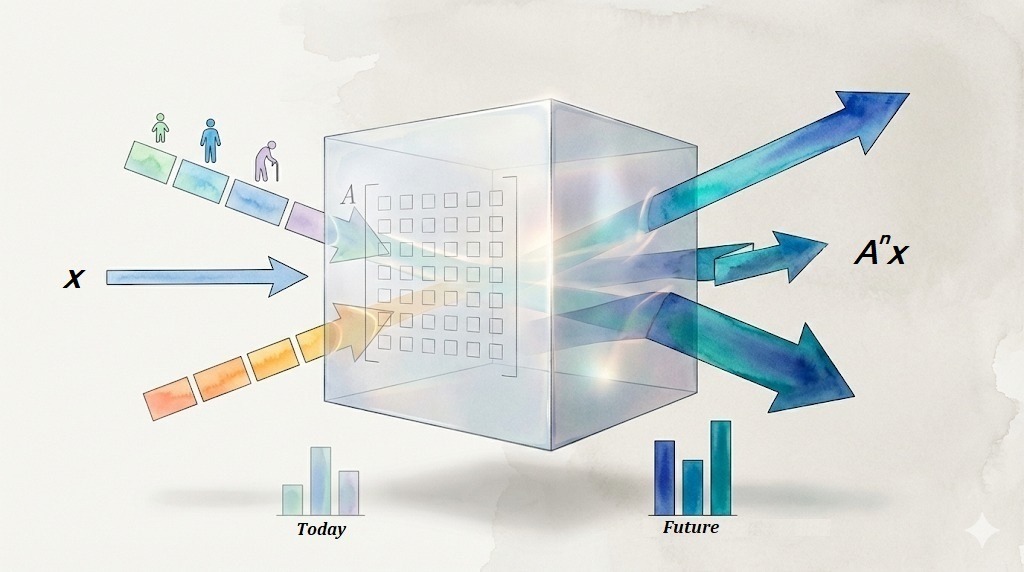
Matrices: Machines Acting On States

A matrix is best thought of as a machine that transforms one state into another. If x is the current state and A is the rule, then the next state is:

x_next = A x

In an age structured population model, let

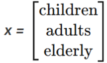
and let A encode birth, survival and transition rates between age groups. Applying A again and again predicts how the population will evolve. The same matrix multiplication that appears in a GATE problem like “Compute A³x” is, in another context, simulating the future of an ecosystem. The algebra has not changed, only the interpretation has.

Rank And Null Space: Freedom Versus Constraints

Consider a linear system

A x = b, A ∈ ℝ^{m × n}.

You are told there are many equations. Intuitively, you expect the solution to be tightly pinned down. Linear algebra quietly asks: how many of these equations are truly independent? That number is the rank of A.

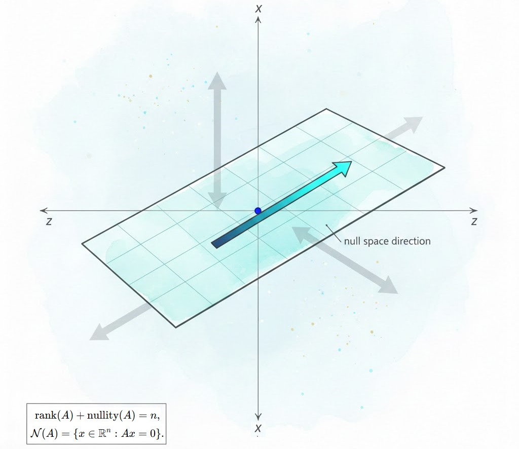
The rank nullity theorem says:

rank(A) + nullity(A) = n

where nullity is the dimension of the null space

N(A) = { x ∈ ℝⁿ : A x = 0 }

Rank measures how many genuine constraints you have. Nullity measures how many directions of motion remain free even after satisfying those constraints. This is why systems with many equations can still have infinitely many solutions. On paper it looks like algebra. In reality it is a negotiation between restriction and freedom.

Eigenvalues: The System’s Preferred Directions

Eigenvalues and eigenvectors come from the equation

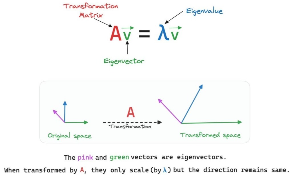
Here v is stretched by a factor λ but its direction is preserved. These directions are the ones that the transformation respects the most. In long term models, one eigenvalue often dominates. In Markov chains, the eigenvector corresponding to eigenvalue 1 describes the steady state distribution. In dimensionality reduction and principal component analysis, eigenvectors of certain matrices reveal the directions in which data varies most.

The surprise comes when a matrix refuses to be simplified. Some matrices cannot be diagonalised. No choice of basis will produce a full set of independent eigenvectors. In exam language: not diagonalizable. In conceptual language: the system does not admit a clean decomposition into independent modes. You are forced to work with Jordan blocks and accept that not every structure has a perfectly neat form.

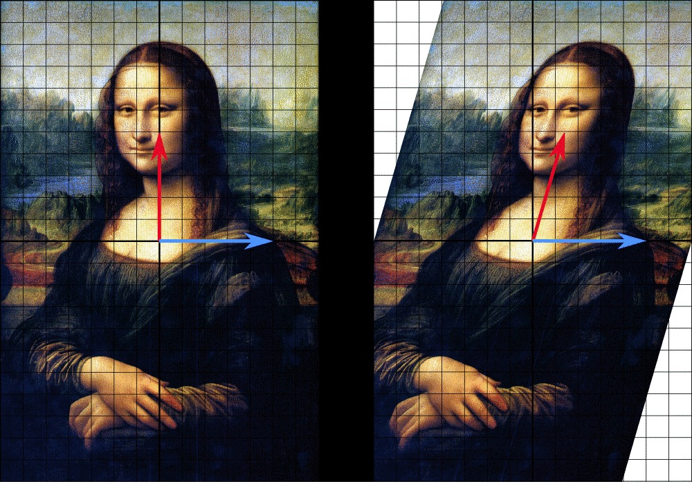
Can you guess which vector among the two is an Eigen Vector?

Projections And Least Squares: When Perfection Is Impossible

Real data rarely fits our equations exactly. For an overdetermined system

A x ≈ b

we look for the vector x that makes the error b − A x as small as possible. The least squares solution x* is defined by the condition:

A^TA x* = A^Tb

Geometrically, Ax ranges over a subspace of ℝ^m. The vector Ax* is the orthogonal projection of b onto this subspace. We do not hit the point exactly, so we choose the closest point allowed by the model.

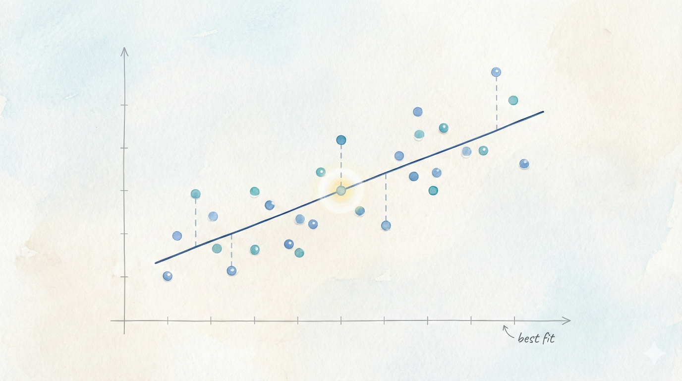
This is the backbone of linear regression, signal denoising and many machine learning algorithms. When you fit a line, you are really computing a projection in a vector space and letting linear algebra decide the fairest compromise.

Linear algebra for GATE is often tested with compact problems. Behind each of those problems stands a way of thinking: states as vectors, rules as matrices, rank as real information, null space as hidden freedom, eigenvectors as preferred directions and projections as intelligent compromise. If you start to see these patterns, the formulas stop being separate topics and start feeling like one coherent language for the structure of the world.

GO Classes Logo